Added the scan of the Pascal user Manual and report Fourth Edition, the ISO standard.
Wirth languages, Pascal, UCSD, Turbo, Delphi, Freepascal, Oberon
The next text and files are by Scott Moore, www.standardpascal.org/p5.html and https://sourceforge.net/p/pascalp5/wiki/Home/
Local copy here.
He deserves all the honours of making this public available! The “I’ is Scott, not me!
Pascal-P5 is available on sourceforge here:
https://sourceforge.net/projects/pascalp5/
Local copy here.
The P5 compiler has existed for a long time as an idea. P4, the last of the Zurich series P-system compilers, left off before the ISO 7185 standard in 1982. It was not only not standard Pascal compliant, it also was only a subset, abeit a substantial one, of full revised Pascal. As an example, or "model" implementation of Pascal, it would have made sense to update the compiler to ISO 7185 status, and that was basically done as "A Model Implementation of Standard Pascal" [Welsh&Hay] before 1986. In fact, the project was designed to support the ISO 7185 project. However, there were a few reasons that a true P5, a straightforward update of the old p4, was a good idea. First, the source code of the "Model Implementation" is not generally available. Second, the "Model Implementation" is a complete scratch rewrite of the compiler, and shares virtually nothing in common with the original P4. This was important because several books, articles and online resources exist for the P4 compiler What I wanted for p5 was a compiler that both accepted ISO 7185 standard Pascal, and was also written in it. The compiler is an extended version of P4 and uses the same intermediate codes where possible. P5 now accepts the full ISO 7185 language, and also has been remade as a byte oriented machine, similar to what was done for both the UCSD compiler and the "Model Implementation". This is is the key to achieving a high efficiency implementation that runs with compact code. P5 also runs the PAT or Pascal Acceptance test, and also self compiles. P5 correctly runs the BSI, or British Standards Institute tests.
P5 is a very important milestone for Pascal. To understand why, it is a good idea to review why P4 was important. P4 was to accomplish:
To understand why P5 is important, you must understand that P4 didn’t completely accomplish the above goals. First of all, P4 was a subset of the full language. It was never designed to run the full language, only a minimal subset that could be ported to a new machine. The idea was to finish out the full language on the target machine.
Unfortunately, that meant there was not a concrete model of some of the more advanced (and hard to implement) features of full Pascal, for example interprocedural gotos, and procedure and function parameters. These and other features of Pascal left out of P4 were often left out of target compilers, and when they were implemented, they were implemented wrong. The other issue is that P4 was designed to be a minimal bootstrap implementation. If you examine P4, you will see that it makes little use of strings, and keeps them short. This is because it is very inefficient when it comes to storing them in memory. They are stored one character to a word (60 bits on the CDC 6000). Pascal has packing, but that is not implemented in P4. Finally, P4 is very much oriented to the CDC 6000 that it originated on. Everything is stored in 60 bit words, and there is a packing system designed to store two instructions per word.
The reason P4 had these limitations is that memory was very limited back in the 1970s, when P4 came about. Even on the CDC 6000. The authors of P4 worked hard to get P4 down in size and memory requirements so that it would self compile. By the time of the ISO 7185 standard, many people understood that P4 was limited for its purposes. The "Model Implementation of Standard Pascal" [Welsh & Hay] was the answer, and it contained a compiler for the full ISO 7185 Pascal language. Further, it implemented the interpreter as a byte oriented machine (sometimes called a "bytecode machine"). Unfortunately, it got sucked up into the BSI, who have effectively killed it (there appear to be no internet copies of it, and the BSI has not been forthcoming concerning it). Another issue with the "Model Implementation" (with apologies to Jim Welsh and Atholl Hay), is that the MI is written in the "self documented" form (avocated by D. E. Knuth and others) where the entire documentation exists in the same file, intermixed with the code. This is a beautiful method to present code as a finished product, but it tends to be fairly difficult to work on an change. Finally, the MI was a complete break with P4, and had nothing in common with it. This meant that MI used completely new methods and documentation, whereas P4 was already documented in the common media and well understood. P5 is both a break with the past and an embrace of it:
The PAT or Pascal acceptance test is a series of tests in one file that go through each feature of ISO 7185 Pascal. If a ISO 7185 Pascal implementation can compile and run this correctly, then it is substantially compliant with ISO 7185 Pascal.
There are two types of tests, the PAT and the PRT, or Pascal Rejection Test. The PAT test should compile and run correctly, and is a "positive" indication that the implementation compiles standard structures and gives standard results. The PRT is the opposite. It is designed to either fail to compile or generate runtime errors or both. It is a "negative" test that makes sure that the implementation rejects non-standard structures. The PAT only is represented here (for now).
The BSI test suite [covered in Wichmann&Ciechanowicz] includes both positive and negative testing, and appeared in original version in the Pascal User’s Group. After a great deal of trouble I was able to OCR a copy of that test, which was published free and clear of restrictions. However, the both the test suite and bore copyright notices at one point, and both were given to the BSI (British Standards Institute) to keep and distribute. The BSI no longer distributes either, at any price, and whether they have kept it is also in doubt. In fact, recently I have been calling them about once a month to find out any information about the pair of programs. Both of them were created at universities outside of the BSI, and both were intended to be distributed, not locked in a vault to be eventually discarded. I don’t and won’t distrubute the BSI test without permission, and I don’t have access to the model compiler. Even with the BSI status of "openly published, but rights kept", I don’t feel comfortable putting it up on this site. However, because it was in fact openly published, I don’t feel that I, as an individual, am unable to run the tests, either. Now, the reason that all of this matters is that with P5, we have effectively replaced the material imprisoned by the BSI. P5 upgrades P4, which never bore a copyright, was public domain, and was distributed openly. I put my own work into upgrading P4 into P5, but I donate that work back to the public domain. As P4 was, P5 is free of copyright and charges. Use as you see fit. The PAT was created entirely by me and is original work. However, I also donate this to public domain. It was created back in the early 1990’s, and used to validate both mine and other Pascal compilers. The PAT effectively replaces the positive testing side of the BSI. I also intend to create a negative test, the PRT, and also make that public domain. Further, the PAT and PRT form a collection point for tests, including test that were made in reaction to the failures seen while running the BSI tests. In other words, if the BSI test found a failure, then an equivalent test was added to the PAT (not copied from the BSI!). This is a work in progress, so not all failure points have yet been addressed. Thus, the PAT and PRT are designed to be full replacements for the BSI tests. Format and working of the PAT The PAT is designed to execute a small amount of code, then print the results. Each "test point" tests one feature of ISO 7185 Pascal,and is numbered according to type and sequence. Here is an example from the test:
  write('Control6: ');
  if true then write('yes') else write('no');
  writeln(' s/b yes');
This prints:
Control 6: yes s/b yes
So you see the number and type of the test, control structures number 6, the result, ‘yes’, and finally what the result should be. The PAT is designed to be verified manually, that is, you read it and check that the printed results equal the "should be" collumn. The PAT can be easily automated for regression purposes by redirecting the output to a file, then comparing a saved "gold" version of the result file to the current file.
P5 is capable compiling itself. This takes different steps for each of the sections, pcom and pint. The resulting intermediate files are listed in the files section below.
I was able to get pcom.pas to self compile. This means to compile and run pcom.pas, then execute it in the simulator, pint. Then it is fed its own source, and compiles itself into intermediate code. Then this is compared to the same intermediate code for pcom as output by the regular compiler. Its a good self check, and in fact found a few bugs.
The Windows batch file to control a self compile and check is:
cpcoms.bat
What does it mean to self compile? For pcom, not much. Since it does not execute itself (pint does that), it is simply operating on the interpreter, and happens to be compiling a copy of itself.
Pint is more interesting to self compile, since it is running (being interpreted) on a copy of itself. Unlike the pcom self compile, pint can run a copy of itself running a copy of itself, etc., to any depth. Of course, each time the interpreter runs on itself, it slows down orders of magnitude, so it does not take many levels to make it virtually impossible to run to completion. Ran a copy of pint running on itself, then interpreting a copy of iso7185pat. The result of the iso7185pat is then compared to the "gold" standard file. As with pcom, pint will not self compile without modification. It has the same issue with predefined header files. Also, pint cannot run on itself unless its storage requirements are reduced. For example, if the "store" array, the byte array that is used to contain the program, constants and variables, is 1 megabyte in length, the copy of pint that is hosted on pint must have a 1 megabyte store minus all of the overhead associated with pint itself. The windows batch file required to self compile pint is:
cpints.bat
As a result, these are the changes required in pint:
{ !!! Need to use the small size memory to self compile, otherwise, by
  definition, pint cannot fit into its own memory. }
maxstr = 2000000; { maximum size of addressing for program/var }
 {maxstr = 200000;} { maximum size of addressing for program/var }

and
{ !!! remove this next statement for self compile }
prd,prr : text;(*prd for read only, prr for write only *)

and
{ !!! remove this next statement for self compile }
reset(prd);

and
{ !!! remove this next statement for self compile }
rewrite(prr);
All these changes were made in the file pintm.pas.
Pint also has to change the way it takes in input files. It cannot read the intermediate from the input file, because that is reserved for the program to be run. Instead, it reads the intermediate from the "prd" header file. The interpreted program can also use the same prd file. The solution is to "stack up" the intermediate files. The intermediate for pint itself appears first, followed by the file that is to run under that (iso7185pat). It works because the intermediate has a command that signals the end of the intermediate file, "q". The copy of pint that is reading the intermediate code for pint
stops, then the interpreted copy of pint starts and reads in the other part of the file. This could, in fact, go to any depth. All of the source code changes from pint.pas to pintm.pas are automated in cpints.bat.
The resulting sizes of the self compiled files are:
pcomm.p5
Storage areas occupied
=====================================
Program             0-114657( 114658)
Stack/Heap   114658-1987994 (1873337)
Constants   1987995-2000000 (  12005)

pintm.p5
Storage areas occupied
=====================================
Program             0- 56194 ( 56195)
Stack/Heap    56195-1993985 (1937791)
Constants     1993986-2000000 ( 6014)
Pascal-P5 is entirely hosted on sourceforge now. Please see the site for all sources:
https://sourceforge.net/projects/pascalp5/
Local copy here.
This lets you access my development link for Pascal-P5. You can use this to:
And much more.
For versioned files (releases) see the files area. The current version is always archived as pascal-p5.tar.gz. The current and previous versions are named as:
pascal-p5_<major version>_<minor version>
That is, each time I create a new version, I make a copy of it using the naming system above. This allows each version to be recovered and used. To get a current development copy of Pascal-P5 source, simply have GIT installed on your system, and execute the following in the directory where you wish to install P5: git clone ssh://samiam95124@git.code.sf.net/p/pascalp5/code pascalp5-code This will get the entire P5 file tree and place it into the target directory "p5".
My common practice is to "bump" the version numer after any changes are made to a certified release. The idea is that the new version number will be the version of the next release to come. This of course can cause confusion. However, the rule, is: if it is not in the above release list, then it is a development version.
For all versions see the readme.txt file in the root directory.
The P5 compiler/assembler is much easier than P4 in one respect. There are no limitations to remember verses ISO 7185 Pascal. If it is legal Standard Pascal, it will compile and run.
To run P5, use the following format:
pcom intermediate.int < source.pas
pint intermediate.int program.out
All files must be specified. This is what the batch file p5.bat given above does.
While upgrading P4 to P5, I specifically tried to avoid any temptation to "improve" the code, such as add functions or features, or reformat the code to be more presentable, etc. There is a time and place for that. I simply wanted P5 to be a full language compiler for Pascal, instead of a subset compiler. The one exception I allowed for is the addition of a routine that dumps all of the error codes that were used in the source compile along with their text equivalents. I have found this to be a great improvement on trying to search the various documents for what error code means what. Of course, virtually all implementations improve on the original Pascal, including the original CDC 6000 compiler. The extensions consist of a combination of features best left defined to a particular implementation, and also usablity extentions to Pascal in general. There’s a lot more that can be done with P5. However, I have left that for the P6 project. P6 is the next step for the P-series, and includes a series of extentions to the base ISO 7185 language.
For more information contact: Scott A. Moore
The Stanford Pascal 360 (1979 version) is a modified version of the P2 Compiler, and except for a few minor extensions, processes the same language. The compiler itself is a 5000 lines Pascal program that translates to P-code. A post processor then translates P-code to IBM assembly code.
The later Stanford Pascal compiler is an offspring of the original Pascal P4 compiler.
A compiler based on the Pascal-P4 compiler, which created native binaries, was released for the IBM System/370 mainframe computer
by the Australian Atomic Energy Commission; it was called the “AAEC Pascal Compiler” after the abbreviation of the name of the Commission.
The AAEC compiler later became the Stanford Pascal compiler (in 1979 ca.), and later again, it was maintained by the McGill university in Montreal, Canada (from 1982 on).
CS-TR-79-731.pdf Stanford Pascal Verifier User Manual, March 1979
TN164_A_Pascal_P-Code_Interpreter_for_the_Stanford_Emmy_Sep79.pdf
October 1974 Stanford Pascal/360 Implementation Guide, contains source of compiler (4665 lines)
pcode_1978.pdf
Stanford1979.pdf
pascal_master.zip many original sources (and later improved versions of Stanford Pascal, part of the Bernd Oppolzer initiative.
Archive with the DECUS DEC PDP-11 Pascal compiler, including sources.
This compiler is a descendent of the ZürichPascal compilers.
            DECUS Pascal for PDP-11
	          ===========================

	          Version 6.3,  November 1985


Abstract:

This compiler implements the Pascal programming language on PDP-11s
running RSX-11 and on other systems that can run RSX tasks (eg. RSTS,
VAX AME).

The main features of this Pascal are:
  - can optionally compile programs to use any arithmetic hardware
  - useful language extensions: default case, loop statement, variable
    length string parameters, substring parameters, structured function
    results, boundless array parameters, and more
  - enhanced I/O facilities for creating and accessing files of
    various types
  - standard file for terminal I/O
  - separate compilation of procedures/functions
  - linkage to external FORTRAN or MACRO routines
  - source "include" facility
  - development aids: statement trace, statement execution profiler,
    conditional compilation
  - high level interactive symbolic debugger and symbolic dump
  - all source and tools provided for maintaining the compiler and
    runtime library (compiler can only be re-compiled on RSX-11).

This release introduces several minor corrections and enhancements.
In particular it now runs on the latest versions of RSTS and RSX.


Restrictions:
Several deviations from the ISO/ANSI Pascal Standard.  (Conformance
report in user manual.)
Automatic Control of Model Helicopter
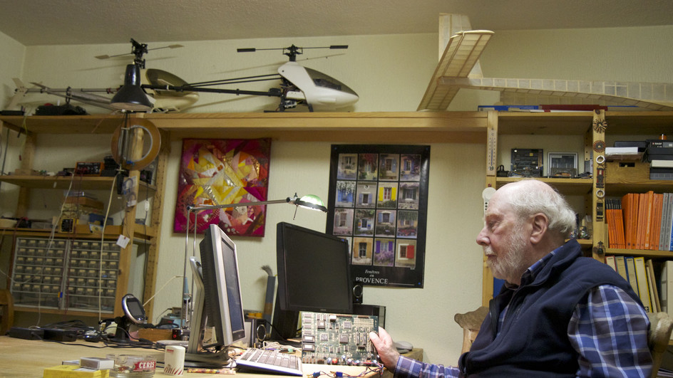
In 1995 Wirth joined a project undertaken at the Institute of Automatic Control and Measurement. The goal was the development of a system to allow a model helicopter to fly autonomously a preprogrammed path. Wirth designed an on-board computer system with a Strong-ARM processor at its core. Aside from the hardware, he also programmed various software tools, including an Oberon subset compiler with additional features for real-time programming. The computer board was built by I. Noack.
The resulting computer system, called Olga, made use of experience with programmable gate arrays, and used the novel Xilinx-Algotronix 6200 fine-grained FPGA for the generation and sensing of pulse-width modulated signals to control the servos. Furthermore, the computer was connected to a compass, a global positioning system (GPS), and a data link via several standard RS-232 interfaces. This system resulted in a drastic reduction of weight and power consumption, and an increase in computing performance compared to the one used before, inspite of the fact that floating-point arithmetic was to be programmed based on integer arithmetic.
The helicopter carrying Olga weighs about 15 kg and is powered by a 35ccm engine. Wirth pushed for a second project based on a downsized helicopter model with a weight of less than 5 kg and a conventional 10ccm engine. This was realized with a considerably smaller computer board, but the same Strong-ARM core and software base. The large FPGA was replaced by several small PLDs. This project, Horla, was confined to the more modest goal of using the computer only to stabilize the inherently unstable craft, while position, speed and direction would remain under remote control by the pilot.
Both projects collected in a remarkable way the various techniques and tools on which Wirth had worked during the past decade: Compiler, operating system, programmable devices (FPGA, PLD) and their design tools including the language Lola, and circuit design in general. Both projects were successful, although only after several years of effort – and patience.
Documents:
Helicopter Flight Control Report 1 The Hardware Core
Helicopter Flight Control Report 2 The Programming Language Oberon SA
Helicopter Flight Control Report 3 The Software Core
Helicopter Flight Control Report 6 The Oberon Compiler for the Strong-ARM Processor
Software for Model Helicopter Flight Control
An Oberon Compiler for the ARM Processor, 2007
/Interrupts and Traps in Oberon-ARM, 2008
SET: A neglected data type, and its compilation for the ARM, 2007
Differences between Revised Oberon and Oberon
The Programming Language Oberon Revision 1.10.2013 / 3.5.2016
Oberon-07 (Revised Oberon) (Oberon at a glance), 2013
Porting the Oberon Compiler from Oberon to Oberon-07, 2007
Lola was designed as a simple, easily learnable hardware description language for describing synchronous, digital circuits. In addition to its use in a digital design course for second year computer science students at ETH Zürich, the Institute for Computer Systems uses it as a hardware description language for describing hardware designs in general and coprocessor applications in particular.
The purpose of Lola is to statically describe the structure and functionality of hardware components and of the connections between them. A Lola text is composed of declarations and statements. It describes the hardware on the gate level in the form of signal assignments. Signals are combined using operators and assigned to other signals. Signals and the respective assignments can be grouped together into types. An instance of a type is a hardware component. Types can be composed of instances of other types, thereby supporting a hierarchical design style and they can be generic (e.g. parametrizable with the word-width of a circuit).
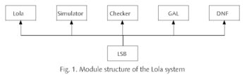
The Lola System is a toolbox consisting of various modules whose commands serve to specify, implement, and test digital circuits. These notes explain its structure to the user of Lola and to the implementer of additional tools. The system’s base is a module containing the definition of the central data structure used to describe digital circuits. Its name is LSB (Lola System Base). Typically, such a data structure is generated from a Lola text by the compiler, and thereafter used as argument for further processing steps, such as simplification, analysis, comparison, simulation, and layout generation. Fig. 1 gives an overview of the described components and their interdependence.
Lola-2: A Logic Description Language, Language description
Lola-2: Translating from Lola to Verilog
Tools for Digital Circuit Design using FPGAs
H Eberle and S. Gehring and S. Ludwig and N.Wirth, 1994
This collection of five papers describes concept and facilities of a system to aid in the design of digital circuits. It is being used in classes and laboratories for circuit design, and also for the development of prototype circuits in research projects. The collection comprises the report on the Lola language for specifying digital circuits, an introduction to field programmable gate arrays (FPGA) and the Atmel 6000 architecture, the user manual of the CL layout editor, the user manual of the CL design checker, and the description of two FPGA extension boards for Ceres-3.
A Laboratory for a Digital Design Course Using FPGAs
Stephan Gehring Stefan Ludwig Niklaus Wirth, 1994
In our digital design laboratory we have replaced the traditional wired circuit modules by workstations equipped with an extension board containing a single FPGA. This hardware is supplemented with a set of software tools consisting of a compiler for the circuit specification language Lola, a graphical layout editor for design entry, and a checker to verify conformity of a layout with its specification in Lola. The new laboratory has been used with considerable success in digital design courses for computer science students. Not only is this solution much cheaper than collections of modules to be wired, but it also allows for more substantial and challenging exercises.
Lola Compiler for Project Oberon, 2013 Edition
LSS.Mod
LSB.Mod
LSP.Mod
LSC.Mod
LSV.Mod
SmallPrograms.Lola
Lola Definition of RISC5 Computer
RISC5.Lola
LeftShifter.Lola
RightShifter.Lola
Multiplier.Lola
Divider.Lola
FPAdder.Lola
FPMultiplier.Lola
FPDivider.Lola
RISC5Top.Lola
PS2.Lola
MouseP.Lola
RS232R.Lola
RS232T.Lola
SPI.Lola
VID.Lola
DCMX3.v
FPGA-related Work
Hardware Design with Field Programmable Gate Arrays (FPGAs), 1990-1999
Similarity and difference between hardware and software design always had intreagued Wirth as a topic. With the emergence of programmable logic devices, the gap between the two fields narrowed. A project to familiarize a team with the new possibilities was established, and research in design methods using the new devices was started. It led to a set of design tools, including a specification language (Debora, B. Heeb), its compiler with several “back ends” for printed circuits boards, PLDs, and FPGAs. The usefulness of these tools was demonstrated by applying them in the construction of a workstation (Chamaeleon, also Ceres-3). The construction process starting from a textual specification and ending with a board layout and PLD programs was automated, and it required almost no manual intervention.
Wirth realized early, that FPGAs would be particularly useful as a field for experimentation in learning digital circuit design, replacing expensive, pluggable circuit modules by programmable cells. He equipped 25 Ceres-3 workstations in a student laboratory with an FPGA and uses them intensively in a digital design class. Along with a new project in tool design went the formulation of his language Lola, specifically tailored to the need of teaching in a systematic manner, dispensing with the myriads of side-issues inherent in commercial HDLs. The tool set consists of a compiler converting the program (circuit) text into an abstract data structure suitable for further processing, an editor for constructing circuits implemented by the FPGA, i.e. for generating a layout, and a checker comparing the specification in Lola with the layout.
The TRM: Experiments in Computer System Design
The Design of a RISC Architecture and its Implementation with an FPGA
– [RISC0.v]
– [RISC0Top.v]
– [PROM.v]
– [DRAM.v]
– [Multiplier.v]
– [Multiplier1.v]
– [Divider.v]
– [RISC0.ucf]
– [RS232R.v]
– [RS232T.v]
StandalonePrograms.Mod
RISC Architecture
Three Counters
The Language PICL and its Implementation, Niklaus Wirth, 20. Sept. 2007
PICL is a small, experimental language for the PIC single-chip microcomputer. The class of computers which PIC represents is characterized by a wordlength of 8, a small set of simple instructions, a small memory of at most 1K cells for data and equally much for the program, and by integrated ports for input and output. They are typically used for small programs for control or data acquisition systems, also called embedded systems. Their programs are mostly permanent and do not change.
All these factors call for programming with utmost economy. The general belief is that therefore programming in a high-level language is out of the question. Engineers wish to be in total control of a program, and therefore shy away from complex languages and compiler generating code that often is unpredictable and/or obscure.
We much sympathize with this reservation and precaution, particularly in view of the overwhelming size and complexity of common languages and their compilers. We therefore decided to investigate, whether or not a language could be designed in such a way that the reservations would be unjustified, and the language would indeed be beneficial for programmers even of tiny systems.
We chose the PIC processor, because it is widely used, features the typical limitations of such single-chip systems, and seems to have been designed without consideration of high-level language application. The experiment therefore appeared as a challenge to both language design and implementation.
The requirements for such a language were that it should be small and regular, structured and not verbose, yet reflecting the characteristics of the underlying processor.
Documents:
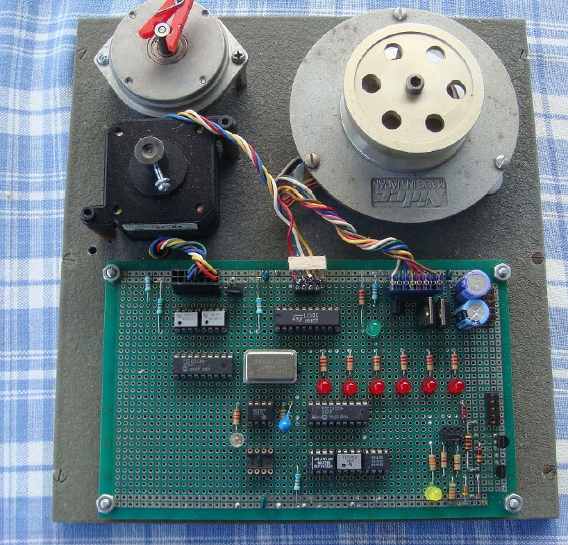
A Microcontroller System for Experimentation, description, parts of which are published on this page.
PICL: A Programming Language for the Microcontroller PIC, EBNF
The Language PICL and its Implementation, Code generation.
PICL Scanner, Oberon source
PICL Parser, Code Generator, Oberon source
The Language PICL
The language is concisely defined in a separate report. Here we merely point out its particular characteristics which distinguish it from conventional languages. Like conventional languages, however, it consist of constant, variable, and procedure declarations, followed by statements of various forms. The simplest forms, again like in conventional languages, are the assignment and the procedure call. Assignments consist of a destination variable and an expression. The latter is restricted to be a variable, a constant, or an operator and its operand pair. No concatenation of operations and no parentheses are provided. This is in due consideration of the PIC’s simple facilities and ALU architecture. Examples can be found in the section on code patterns below. Conditional and repetitive statements are given the modern forms suggested by E. W. Dijkstra. They may appear as somewhat cryptic. However, given the small sizes of programs, this seemed to be appropriate.
Conditional statements have the form shown at the left and explained in terms of conventional notation to the right.
[cond -> StatSeq]                     IF cond THEN Statseq END
[cond -> StatSeq0|* StatSeq1 ]        IF cond THEN Statseq0 ELSE StatSeq1 END
[cond0 -> StatSeq0|cond1 -> StatSeq1] IF cond0 THEN Statseq0 ELSIF cond1 THEN StatSeq1END
Repetitive statements have the form:
{cond -> StatSeq}                     WHILE cond DO Statseq END
{cond0 -> StatSeq0|cond1 -> StatSeq1} WHILE cond0 DO Statseq0 ELSIF cond1 DO StatSeq1END
There is also the special case mirroring a restricted form of for statement. Details will be
explained in the section on code patterns below.
{| ident, xpression -> StatSeq}
The PICL Compiler
The compiler consists of two modules, the scanner, and the parser and code generator. The scanner recognizes symbols in the source text. The parser uses the straight-forward method of syntax analysis by recursive descent. It maintains a linear list of declared identifiers for constants, variables, and procedures.
Example
MODULE RepeatStat;
  INT x, y;
BEGIN
  REPEAT x := x + 10; y := y - 1 UNTIL y = 0;
  REPEAT DEC y UNTIL y = 0
END RepeatStat.

0 0000300A MOVLW 10
1 0000078C ADDWF 1 12 x := x + 10
2 00003001 MOVLW 1
3 0000028D SUBWF 1 13
4 0000080D MOVFW 0 13 y := y - 1
5 00001D03 BTFSS 2 3 = 0 ?
6 00002800 GOTO 0
7 00000B8D DECFSZ 1 13 y := y – 1; = 0?
8 00002807 GOTO 7
Example
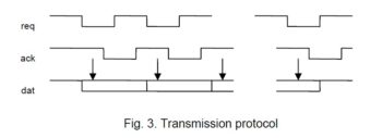
The following procedures serve for sending and receiving a byte. Transmission occurs over a 3-wire connection, using the conventional hand-shake protocol. Port A.3 is an output. It serves for signaling a request to receive a bit. Port B.6 is an input and serves for transmittithe data. B.7 is usually in the receiving mode and switched to output only when a byte is to be sent. In the idle state, both request and acknowledge signals are high (1).
PROCEDURE Send(INT x);
  INT n;
BEGIN ?B.6;                     wait for ack = 1
  !S.5; !~B.7; !~S.5; n := 8;   switch B.7 to output
  REPEAT
    IFx.0 -> !B.7 ELSE !~B.7 END; apply data
    !~A.3; issue request
    ?~B.6; wait for ack
    !A.3; ROR x; reset req, shift data
    ?B.6; DEC n wait for ack reset
  UNTIL n = 0;
  !S.5; !B.7;!~S.5 reset B.7 to input
END Send;

PROCEDURE Receive;
  INT n;
BEGIN d := 0; n := 8; result to global vaiable d
  REPEAT
    ?~B.6; ROR d;     wait for req
    IF B.7 THEN !d.7 ELSE !~d.7 END ; sense data
    !~A.3;           issue ack
    ?B.6;            wait for req reset
    !A.3; DEC n      reset ack
  UNTIL n = 0
END Receive;
Another version of the same procedures also uses three lines. But it is asymmetric: There is a master and a slave. The clock is always delivered by the master on B.6 independent of the direction of the data transmission on A3 and B7.
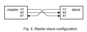
When sending, the data is applied to A.3, when receiving, the data is on B.7. The advantage of this scheme is that no line ever switches its direction, the disadvantage is its dependence on the relative speeds of the two partners. The clock must be sufficiently slow so that the slave may follow. There is no acknowledgement.
Master                              Slave
PROCEDURE Send(INT x);              PROCEDURE Receive;
  INT n;                              INT n;
BEGIN n := 8;                       BEGIN d := 0; n := 8;  result to global vaiable d
  REPEAT                              REPEAT ?~B.6; !>d;   wait for clock low
    IF x.0 THEN !A.3 ELSE !~A.3 END;    IF B.7 THEN !d.7 ELSE ~d.7 END; sense data
    !~B.6; !>x; !B.6; DEC n             ?B.6; DEC n        wait for clock high
  UNTIL n = 0                         UNTIL n = 0
END Send;                           END Receive;

PROCEDURE Receive;                  PROCEDURE Send(INT x);
  INT n;                              INT n;
BEGIN d := 0; n := 8;               BEGIN n := 8;
  REPEAT !~B.6; ROR d;                REPEAT ?~B.6;        wait for clock low
    IF B.7 THEN !d.7 ELSE ~d.7 END;     IF x.0 THEN !A.3 ELSE !~A.3 END; apply data
    !B.6; DEC n                         ROR x ?B.6; DEC n  wait for clock high
  UNTIL n = 0                         UNTIL n = 0
END Receive;                        END Send;
Conclusions
The motivation behind this experiment in language design and implementation had been thequestion: Are high-level languages truly inappropriate for very small computers? The answer is: Not really, if the language is designed in consideration of the stringent limitations. I justify my answer out of the experience made in using the language for some small sample programs. The corresponding assembler code is rather long, and it is not readily understandable. Convincing oneself of its correctness is rather tedious (and itself error-prone). In the new notation, it is not easy either, but definitely easier due to the structure of the text.
In order to let the regularity of this notation stand out as its main characteristic, completeness was sacrificed, that is, a few of the PIC’s facilities were left out. For example, indirect addressing, or adding multiple-byte values (adding with carry). Corresponding constructs can easily be added.
One might complain that this notation is rather cryptic too, almost like assembler code. However, the command (!) and query (?) facilities are compact and useful, not just cryptic. Programs for computers with 64 bytes of data and 2K of program storage are inherently short; their descriptions should therefore not be longwinded. After my initial doubts, the new notation appears as a definite improvement over conventional assembler code.
The compiler was written in the language Oberon. It consists of a scanner and a parser module of 2 and 4 pages of source code respectively (including the routines for loading and verifying the generated code into the PIC’s ROM). The parser uses the time-honored principle of top-down, recursive descent. Parsing and code generation occur in a single pass.
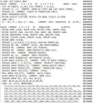
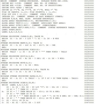
Euler is a programming language created by Niklaus Wirth and Helmut Weber, conceived as an extension and generalization of ALGOL 60. The designers’ goal was to create a language which was simpler, and yet more flexible, than ALGOL 60 that was a useful programming language processed with reasonable efficiency that can be defined with rigorous formality. Available sources indicate that Euler was operational by 1965.
Euler employs a general type concept. In Euler, arrays, procedures, and switches are not quantities which are declared and named by identifiers: they are not (as opposed to ALGOL) quantities which are on the same level as variables, rather, these quantities are on the level of numeric and boolean constants. Thus, besides the traditional numeric and logical constants, Euler introduces the following additional types:
All constants can be assigned to variables, which have the same form as in ALGOL, but for which no fixed types are specified: Euler is a dynamically typed programming language. Furthermore, a procedure can produce a value of any type when executed, and this type can vary from one call of the procedure to the next. Similarly, the elements of a list can have values of any type and these can be different from element to element within the list. So, when the list elements are labels, a switch is obtained. If the elements are procedures, a procedure list is obtained (which is not available in ALGOL 60). If the elements are lists themselves, then a general tree structure is obtained. Euler provides general type-test and type-conversion operators.
Sample program
BEGIN NEW FOR; NEW MAKE; NEW T; NEW A;
FOR ~ LQ FORMAL CV; FORMAL LB; FORMAL STEP; FORMAL UB; FORMAL S;
BEGIN
LABEL L; LABEL K;
CV ~ LB;
K: IF CV { UB THEN S ELSE GOTO L;
CV ~ CV + STEP;
GOTO K;
L: 0
END RQ;
MAKE ~ LQ FORMAL B; FORMAL X;
BEGIN NEW T; NEW I; NEW F; NEW L;
L ~ B; T ~ LIST L[1];
F ~ IF LENGTH L ! 1 THEN MAKE(TAIL L, X) ELSE X;
FOR (@I, 1, 1, L[1], LQ T[I] ~ F RQ);
T
END RQ;
A ~ ();
FOR (@T, 1, 1, 4, LQ BEGIN A ~ A &amp;amp; (T); OUT MAKE(@A,T) END RQ)
END $
DUMP
Downloads:
|
EULER Formal Definition, Niklaus Wirth |
|
Source of EULER, 1965 |
|
Syntax Processor, Nikluas Wirth, 1964 |
|
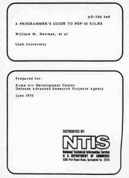
PDP10 EULER handbook |
|
EULER An Experiment in Language Definiton, Thomas W. Cristopher |
See also for an Icon implementation of an Euler compiler/interpreter
PROGRAM
BLOCK
BLOKHEAD
BLOKBODY
LABDEF
STAT
STAT-
EXPR
EXPR-
IFCLAUSE
TRUEPART
CATENA
DISJ
DISJHEAD
CONJ
CONJ-
CONJHEAD
NEGATION
RELATION
CHOICE
CHOICE-
SUM
SUM-
TERM
TERM-
FACTOR
FACTOR-
PRIMARY
PROCDEF
PROCHEAD
LIST*
LISTHEAD
REFERENC
NUMBER
REAL*
INTEGER*
INTEGER-
DIGIT
LOGVAL
VAR
VAR-
VARDECL
FORDECL
LABDECL
*
0
1
2
3
4
5
6
7
8
9
,
.
;
:
@
NEW
FORMAL
LABEL
IDENT*
[
]
BEGIN
END
(
)
LQ
RQ
GOTO
OUT
~
IF
THEN
ELSE
&amp;amp;
OR
AND
NOT
=
!
&amp;lt;
{
}
&amp;gt;
MIN
MAX
+
-
|
/
%
MOD
*
ABS
LENGTH
INTEGER
REAL
LOGICAL
LIST
TAIL
IN
ISB
ISN
ISR
ISL
ISLI
ISY
ISP
ISU
SYMBOL*
UNDEFINE
TEN
#
TRUE
FALSE
$
*
VARDECL NEW IDENT* 001
FORDECL FORMAL IDENT* 002
LABDECL LABEL IDENT* 003
VAR- IDENT* 004
VAR- VAR- [ EXPR ] 005
VAR- VAR- . 006
VAR VAR- 007
LOGVAL TRUE 010
LOGVAL FALSE 011
DIGIT 0 012
DIGIT 1 013
DIGIT 2 014
DIGIT 3 015
DIGIT 4 016
DIGIT 5 017
DIGIT 6 020
DIGIT 7 021
DIGIT 8 022
DIGIT 9 023
INTEGER- DIGIT 024
INTEGER- INTEGER- DIGIT 025
INTEGER* INTEGER- 026
REAL* INTEGER* . INTEGER* 027
REAL* INTEGER* 030
NUMBER REAL* 031
NUMBER REAL* TEN INTEGER* 032
NUMBER REAL* TEN # INTEGER* 033
NUMBER TEN INTEGER* 034
NUMBER TEN # INTEGER* 035
REFERENC @ VAR 036
LISTHEAD LISTHEAD EXPR , 037
LISTHEAD ( 040
LIST* LISTHEAD EXPR ) 041
LIST* LISTHEAD ) 042
PROCHEAD PROCHEAD FORDECL ; 043
PROCHEAD LQ 044
PROCDEF PROCHEAD EXPR RQ 045
PRIMARY VAR 046
PRIMARY VAR LIST* 047
PRIMARY LOGVAL 050
PRIMARY NUMBER 051
PRIMARY SYMBOL* 052
PRIMARY REFERENC 053
PRIMARY LIST* 054
PRIMARY TAIL PRIMARY 055
PRIMARY PROCDEF 056
PRIMARY UNDEFINE 057
PRIMARY [ EXPR ] 060
PRIMARY IN 061
PRIMARY ISB VAR 062
PRIMARY ISN VAR 063
PRIMARY ISR VAR 064
PRIMARY ISL VAR 065
PRIMARY ISLI VAR 066
PRIMARY ISY VAR 067
PRIMARY ISP VAR 070
PRIMARY ISU VAR 071
PRIMARY ABS PRIMARY 072
PRIMARY LENGTH VAR 073
PRIMARY INTEGER PRIMARY 074
PRIMARY REAL PRIMARY 075
PRIMARY LOGICAL PRIMARY 076
PRIMARY LIST PRIMARY 077
FACTOR- PRIMARY 100
FACTOR- FACTOR- * PRIMARY 101
FACTOR FACTOR- 102
TERM- FACTOR 103
TERM- TERM- | FACTOR 104
TERM- TERM- / FACTOR 105
TERM- TERM- % FACTOR 106
TERM- TERM- MOD FACTOR 107
TERM TERM- 110
SUM- TERM 111
SUM- + TERM 112
SUM- - TERM 113
SUM- SUM- + TERM 114
SUM- SUM- - TERM 115
SUM SUM- 116
CHOICE- SUM 117
CHOICE- CHOICE- MIN SUM 120
CHOICE- CHOICE- MAX SUM 121
CHOICE CHOICE- 122
RELATION CHOICE 123
RELATION CHOICE = CHOICE 124
RELATION CHOICE ! CHOICE 125
RELATION CHOICE &amp;lt; CHOICE 126
RELATION CHOICE { CHOICE 127
RELATION CHOICE } CHOICE 130
RELATION CHOICE &amp;gt; CHOICE 131
NEGATION RELATION 132
NEGATION NOT RELATION 133
CONJHEAD NEGATION AND 134
CONJ- CONJHEAD CONJ- 135
CONJ- NEGATION 136
CONJ CONJ- 137
DISJHEAD CONJ OR 140
DISJ DISJHEAD DISJ 141
DISJ CONJ 142
CATENA CATENA &amp;amp; PRIMARY 143
CATENA DISJ 144
TRUEPART EXPR ELSE 145
IFCLAUSE IF EXPR THEN 146
EXPR- BLOCK 147
EXPR- IFCLAUSE TRUEPART EXPR- 150
EXPR- VAR ~ EXPR- 151
EXPR- GOTO PRIMARY 152
EXPR- OUT EXPR- 153
EXPR- CATENA 154
EXPR EXPR- 155
STAT- LABDEF STAT- 156
STAT- EXPR 157
STAT STAT- 160
LABDEF IDENT* : 161
BLOKHEAD BEGIN 162
BLOKHEAD BLOKHEAD VARDECL ; 163
BLOKHEAD BLOKHEAD LABDECL ; 164
BLOKBODY BLOKHEAD 165
BLOKBODY BLOKBODY STAT ; 166
BLOCK BLOKBODY STAT END 167
PROGRAM $ BLOCK $ 170
*
PL360 (or PL/360) is a system programming language designed by Niklaus Wirth and written by Niklaus Wirth, Joseph W. Wells, Jr., and Edwin Satterthwaite, Jr. for the IBM System/360 computer at Stanford University. A description of PL360 was published in early 1968.
Niklaus Wirth in 1966 wanted to have a compiler written for his new Algol W language and the choices of programming language with which to write the compiler were FORTRAN and assembler language Wirth set aside the Algol W project temporarily and developed a programming language which was specifically designed for writing system-level software on an IBM 360 system. This systems programming language, the very first systems programming language other than assembler language, came to be known as PL360 (the name is sometimes written as PL/360 although it seems pretty clear that Wirth called it PL360 – I’m not 100% sure of this so please correct me if I’m wrong).
In practical terms, PL360 isn’t much more than an assembly language dressed up in fancy clothes (strictly speaking, it’s actually called a structured assembly language). Although a reasonable set of operators are defined, expression evaluation is strictly left to right and the programmer is responsible for managing the use of the machine registers and most aspects of memory management. In fact, it really wasn’t possible to write a PL360 program without quite intimate knowledge of the System/360 architecture.
The result is a language which requires considerable care and attention on the part of the programmer. Although friendlier than an actual assembler language, the inattentive programmer is provided with plenty of potential learning opportunities (i.e. pitfalls). For example, consider the following two statements:
R1 := R1 + R2;
R1 := R2 + R1;
Although these may appear to be equivalent, they are actually VERY different. The first statement adds machine register R2 to the contents of register R1 and stores the result in R1 (i.e. it adds R1 and R2 together and stores the result in R1). The second statement is actually equivalent to:
R1 := R2; R1 := R1 + R1;
i.e. it effectively computes 2*R2 and stores the result in R1.
PL360 ends up looking pretty sad if it is considered as a high-level programming language. On the other hand, if viewed as a mid to low-level language (i.e. an assembler language in fancy clothes) then it was actually quite respectable for the era. In fact, since the goal was to create a language which could be used to do systems programming, the necessity to understand the underlying architecture in detail was arguably a language feature rather than a failing.
By 1968, a compiler had been written for the PL360 language and Wirth was able to get on with the task of getting an Algol W compiler written. The ability to write systems programming level software using reasonably conventional looking statements and expressions turned out to be quite useful and PL360 went on to be used for a variety of projects.
PL/360 is a one pass compiler with a syntax similar to Algol that provides facilities for specifying exact machine language instructions and registers similar to assembly language, but also provides features commonly found in high-level languages, such as complex arithmetic expressions and control structures. Wirth used PL360 to create Algol W.
Data types are:
From the CS33 Stanford University Report: A Programming Language for the 36O Computers, Niklaus Wirth, Introduction
This paper is a preliminary definition of a programming language which is specifically designed for use on IBM 360 computers, and is therefore appropriately called PL36O.
The intention is to present a programming tool which (a) closely reflects the particular structure of the 36O computer, and (b) is a superior notation to present Assembly Codes with respect to presentation and documentation of algorithms. As a consequence of (a), it enables a programmer to design programs mentioning explicitly features of this machine in a degree impossible in “higher level” languages.
It is also felt that a highly structured language is most appropriate (a) to promote the intelligibility of texts for the human user and (b) to encourage this user to properly structure his algorithms not on paper only, but in his mind as well. The language is therefore a phrase structure language containing many constructions which quite obviously correspond to a single 36O machine instruction (cf, [l]).
Moreover, it is hoped that through certain conventions (not mentioned in this preliminary paper) concerning the use of general registers as base address registers, programs written in PL36O can be efficiently run under a time-sharing monitor without requiring the presence of additional sophisticated relocation hardware (Model 67)°
Presently, a compiler for PL36O is available on the B55OO computer
This compiler is mainly intended to serve as a temporary tool for a bootstrapping process: The compiler is being rewritten in its own language and then becomes automatically available on the 36O computer. Indeed, the primary purpose of this project is to obtain a convenient tool for the development of other compilers (in particular ALGOL X) and monitor systems, where a considerable degree of machine-orientation and -dependence is desirable, but where an adequate standard of program documentation is of no less importance.
Documents for download:
During his stay at Stanford University Wirth designed ALGOL W, his first widely distributed structured language. He first implemented PL/360 , the structured assembler for the IBM 360 architecture, to have a development system for ALGOL-W.
ALGOL W is a programming language, based on a proposal for ALGOL X by Niklaus Wirth and Tony Hoare as a successor to ALGOL 60 in the International Federation for Information Processing (IFIP) IFIP Working Group 2.1. When the committee decided that the proposal was not a sufficient advance over ALGOL 60, the proposal was published as A contribution to the development of ALGOL.
After making small modifications to the language Wirth supervised a high quality implementation for the IBM/360 at Stanford University that was widely distributed.
It represented a relatively conservative modification of ALGOL 60, adding string, bitstring, complex number and reference to record datatypes and call-by-result passing of parameters, introducing the while statement, replacing switch with the case statement, and generally tightening up the language. The implementation was written in PL/360, an ALGOL-like assembly language designed by Wirth. The implementation includes influential debugging and profiling abilities.
ALGOL W’s syntax is built on a subset of the EBCDIC character set. In ALGOL 60 reserved words are distinct lexical items, but in ALGOL W they are merely sequences of characters, and do not need to be stropped. Reserved words and identifiers are separated by spaces. In these ways ALGOL W’s syntax resembles that of Pascal and later languages.
The Algol W Language Description (see below)defines Algol W in an affix grammar that resembles BNF. This grammar was a precursor of the Van Wijngaarden grammar.
Much of Algol W’s semantics is defined grammatically: Identifiers are distinguished by their definition within the current scope. For example, a ⟨procedure identifier⟩ is an identifier that has been defined by a procedure declaration, a ⟨label identifier⟩ is an identifier that is being used as a goto label. The types of variables and expressions are represented by affixes. For example ⟨τ function identifier⟩ is the syntactic entity for a function that returns a value of type τ, if an identifier has been declared as an integer function in the current scope then that is expanded to ⟨integer function identifier⟩. Type errors are grammatical errors. For example “⟨integer expression⟩ / ⟨integer expression⟩” and “⟨real expression⟩ / ⟨real expression⟩” are valid but distinct syntactic entities that represent expressions, but “⟨real expression⟩ DIV ⟨integer expression⟩” (i.e. integer division performed on a floating-point value) is an invalid syntactic entity.
The major part of ALGOL W, amounting to approximately 2700 cards (see listing below), was written in Wirth’s PL360. An interface module for the IBM operating system in use (OS, DOS, MTS, ORVYL) was written in IBM assembler, amounting to fewer than 250 cards. In an OS environment on a 360/67 with spooled input and output files, the compiler will recompile itself in about 25 seconds. The compiler is approximately 2700 card images. Thus, when the OS scheduler time is subtracted from the execution time given above, it is seen that the compiler runs at a speed in excess of 100 cards per second (for dense code). In a DOS environment on a 360/30, the compiler is limited only by the speed of the card reader. The compiler has successfully recompiled itself on a 64K 360/30 at a rate of 1200 cards per minute (the speed of the card reader).
Documents for download:
If you want to work with ALGOL-W, there is a recent implementation AWE for Linux (and Windows via CYGWIN) .
From https://everything2.com/title/Algol+W
In the early 1960s, the IFIP Working Group 2.1 committee was created with the mandate to design a language to replace Algol+60. By the time of the regular committee meeting in the fall of 1966, there were three competing proposals on the table. One of the proposals, by Niklaus Wirth, was for a language which was a relatively modest improvement over Algol 60. One of the other proposals, by Van Wijngaarden, was chosen by the committee and was to evolve into Algol 68. As a result of the decision to pursue Van Wijngaarden’s proposal, a number of the committee members, including Wirth and C.A.R. Hoare, abandoned the committee (it was, apparently, a pretty intense meeting). Wirth developed his proposal into an Algol-style language which, eventually, came to be known as Algol W (like Algol 60 before it, the Algol W language’s gramma was formally described using BNF notation). Although less ambitious than Van Wijngaarden’s proposal, Wirth’s language introduced a number of new concepts including:
When it came time to actually compiler for the language, a decision was made to first develop a systems programming language called PL360 (the only real alternatives were FORTRAN and Assembler). Once a PL360 compiler had been written, it was used (in about 1968) to implement an Algol W compiler on the OS/360 and MTS (Michigan Terminal system) operating systems.
Algol W was reasonably successful as a teaching language although it was rarely if ever used in commercial contexts. By about 1980, Algol W was being replaced by languages like Pascal.
The following is a brief description of the language as it was defined in 1972.
Algol W dates back to the days of punched cards. Consequently, the language is defined strictly in terms of upper case. For example, the following is a valid Algol W program
BEGIN
WRITE("Hello world");
END.
but the following is not
begin
write("Hello world");
end.
Like C, statements are terminated by a semi-colon and whitespace can appear anywhere except within an identifier or reserved word.
The reserved words are
ABS
ALGOL (used when writing separately compiled ‘modules’)
AND
ARRAY
ASSERT
BEGIN
BITS
CASE
COMMENT
complex number COMPLEX
DIV
DO
ELSE
EEND
FALSE
FOR
FORTRAN (used to call a separately compiled FORTRAN routine)
GO TO
GOTO
IF
INTEGER
IS
LOGICAL” LOGICAL
LONG
NULL
OF
OR
PROCEDURE
REAL
RECORD
REFERENCE
REM
RESULT
SHL
SHORT
SHR
STEP
STRING
THEN
TRUE
UNTIL
VALUE
WHILE
The following is the list of data types supported by the language. Example declarations and constants are provided for each data type.
INTEGER I, J;
10
1232
REAL W, X;
10.
10.0
0.1
.1
LONG REAL Y, Z;
10.L
10.0L
0.1L
.1L
10L
COMPLEX A, B;
10.I
10.0I
0.1I
.1I
10I
Note that the complex constant only represents the imaginary part of the number. A specification of a complete complex value would involve the addition of a real value with a complex value. e.g. 5.0 + 3I or 7 + 3I (the integer constant 7 would be automatically converted to the real value 7.0 before it was added to the complex constant value 3i).
COMPLEX C, D;
10.IL 10.0IL 0.1IL .1IL 10IL
LOGICAL E, F;
TRUE
FALSE
BITS G, H;
#001248CF
Note that bits constants are represented in hexadecimal. The above constant is equivalent to the binary value 00000000000100100100100011001111.
STRING S; STRING(40) T;
"hello"        a string containing the 5 characters h, e, l, l and o
""""           a string containing a single "
All strings are fixed length with a minimum length of 1 and a maximum length of 256. If the length isn’t specified in a STRING declaration then it defaults to 16. Also note that there is no backslash convention as is found in many “modern” languages. Use two double quotes in a row if you want to have a single double quote within a string constant.
RECORD PERSON( STRING(40) NAME; INTEGER AGE; REAL HEIGHT );
PERSON( "DANIEL BOULET", 45, 180.3 )
PERSON
The PERSON( “DANIEL BOULET”, 45, 180.3 ) example defines
a new PERSON RECORD and initializes all the fields. The second PERSON example creates a new PERSON RECORD with the field
values uninitialized. Neither of these examples are really constants.
REFERENCE (PERSON) DANIEL; REFERENCE (PERSON,THING) IT;
NULL
Algol W also supports arrays which can be constructed using any of the other data types. Here are a few example declarations:
INTEGER ARRAY VECTOR(1::10);         COMMENT ten element array of integers;
REAL    ARRAY MATRIX(1::10,1::10);   COMMENT a square 10x10 array of reals;
INTEGER ARRAY RANGE(-10::10);        COMMENT a 21 element array (-10 to +10);
REFERENCE(THING) ARRAY THINGS(1::N); COMMENT an array of references to
                                             things with a size determined
					     at run-time;
Any of the bounds of an array declaration can be an expression which is evaluated at run-time. If the result is an array in which the lower bound is greater than the upper bound (for any dimension) then the array has no elements – i.e. any attempt to access the array will result in a run-time array bounds error.
Examples for each of the above arrays are:
WRITE( VECTOR(1) );           COMMENT print out first element of VECTOR;
MATRIX(10,1) := MATRIX(1,10); COMMENT copy an element of MATRIX;
RANGE(0) := 0;                COMMENT set the middle element of RANGE to 0;
WRITE(NAME(THINGS(1)));       COMMENT write out the value of the NAME field of the first THING;
Algol W supports the usual set of operators although it distinguishes between integer and non-integer division operators.
The operators are:
OR
AND
¬
< <= = ¬= >= > IS
+ -
* / DIV REM
SHL SHR **
LONG SHORT ABS
A few notes are in order:
IF IT IS PERSON THEN
   WRITE("IT is pointing at a PERSON record")
ELSE
   WRITE("IT is not pointing at a PERSON record");
Parentheses can, of course, be used to override the operator precedence. Missing from the above list is the unary – and + operators which have higher precendence than any of the binary operators. Missing from this entire writeup is a description of the reasonably large (for the era) set of built-in library routines. Also missing from the above list is a mechanism to access fields of a RECORD. The syntax for this is identical to a function call where the name of the function is the name of the field and the single parameter to the call is the REFERENCE variable. For example,
AGE(DANIEL) := AGE(DANIEL) + 1;
would increment the AGE field of the PERSON record referenced by DANIEL.
Here’s a very short example program
BEGIN
INTEGER I, J, PRODUCT;
READ(I,J);  COMMENT read two integers from the input device;
PRODUCT := I * J; WRITE("The product is ",PRODUCT);
END.
A few notes are in order
Everything up to the next semi-colon is ignored
This allows it to be distinguished from the comparison for equality operator which is =.
Like all Algol languages, Algol W is a block structured language. This means that the scope of an identifier is determined by the block within which it is declared. For example, the output of the following program
BEGIN
INTEGER I;
I := 10;
WRITE("I is ",I);
   BEGIN
   INTEGER I;
   I := 20;
   WRITE("this I is ",I);
   END;
WRITE("I is still ",I);
   BEGIN
   I := 30;
   WRITE("I is now ",I);
   END;
WRITE("I's final value is ",I);
END.
would be
I is 10
this I is 20
I is still 10
I is now 30
I's final value is 30
The scope of the I declared on the second line is the entire program except for the first inner block which has a different I declared within it.
Algol W has function procedures and proper procedures. A function procedure returns a value and can be used in any context in which an expression can appear. A proper procedure does not return a value. Today, these are generally called functions and procedures respectively. Procedures of either kind can be defined to accept parameters. Here are a pair of examples:
BEGIN
INTEGER P, Q;

PROCEDURE PROC( INTEGER VALUE I, J; INTEGER RESULT PRODUCT );
   BEGIN
   WRITE("call to PROC - I is ",I,", J is ",J,".");
   PRODUCT := I * J;
   END;

INTEGER PROCEDURE FUNC( INTEGER VALUE I, J );
    BEGIN
    WRITE("call to FUNC - I is ",I,", J is ",J,".");
    I * J
    END;

PROC(10, 20, P);
Q := FUNC(10, 20);
END.
The first is a proper procedure called PROC which takes two integer parameters which are initialized based on the first two arguments passed on the call to PROC (i.e. I is initialized to 10 and J is initialized to 20 in this example). It returns a result parameter PRODUCT (i.e. P will be assigned 200 just as the call to PROC returns).
The second is a function procedure called FUNC which takes two integer parameters and returns their product as the value of the procedure (the last thing before the closing END in a function procedure’s body must be an expression which is evaluated to compute the value of the procedure).
Here’s an example of a function procedure that takes no parameters:
BEGIN
INTEGER Q;

REAL PROCEDURE ZERO;
   BEGIN
   0
   END;

Q := ZERO;
END.
This is an expensive (and absurd) way to initialize Q to 0. Short procedures consisting of a single statement can dispense with the BEGIN-END block:
PROCEDURE HELLO;
    WRITE("Hello");
Algol W, like its predecessor Algol 60, also supports the call by name parameter passing mechanism:
BEGIN
INTEGER J;
PROCEDURE BYNAME(INTEGER MAGIC);
   BEGIN
   WRITE("MAGIC is ",MAGIC);
   J := J * 2;
   WRITE("MAGIC is now ",MAGIC);
   END;
J := 10;
BYNAME(J * 3);
END.
A call by name parameter is re-evaluated every time it is used. Consequently, the output of the above program would be:
MAGIC is 30
MAGIC is now 60
The potential for, shall we say, strange program behaviour when using call by name is great enough that the mechanism is rarely used.
A binary operator which combines the value of two function calls, at least one of which modifies a global variable and the other of which relies upon the same global variable, produces unpredictable results. For example, the output of the following program
BEGIN
INTEGER J;
INTEGER PROCEDURE LEFT;
   BEGIN
   J := J + 1;
   J
   END;
INTEGER PROCEDURE RIGHT;
   BEGIN
   J := J * 3;
   J
   END;
J := 2;
WRITE( LEFT * RIGHT );
END.
might be 27 or 42 depending on which of LEFT or RIGHT is called first when the operands of the * operator in the WRITE call are evaluated.
Like all the Algol languages, Algol W supports recursion. Here’s an excellent way to consume vast quantities of CPU time:
INTEGER PROCEDURE ACKERMANN(INTEGER VALUE X, Y);
    IF X = 0 THEN
	Y + 1
    ELSE IF Y = 0 THEN
	ACKERMANN(X - 1, 1)
    ELSE
	ACKERMANN(X - 1, ACKERMANN(X, Y - 1));
If you want to find out if your computer can stay up for a few thousand millennium, call this function with
ACKERMANN(1000,1000)
Although apparently not part of the original language, the 1972 version of Algol W supports block expressions. This is a generalization of how function procedure bodies are written.
It allows the following sort of nonsense to be written:
BEGIN
WRITE("the answer is ",
   BEGIN
   INTEGER X;
   X := 2 * 3;
   X
   END
   * 7
);
END.
In practical terms, block expressions aren’t used very often as they tend to make the program harder to read without adding any real value. Block expressions which modify global variables can also produce unpredictable results:
BEGIN
INTEGER J;
J := 2;
WRITE(
   BEGIN
   J := J + 1;
   J
   END
   *
   BEGIN
   J := J * 3;
   J
   END
);
END.
This program is equivalent to the example given above involving the function procedures LEFT and RIGHT.
The IF statement is used to conditionally execute a single statement:
IF I > 10 THEN
   I := I * 2;
An ELSE clause can be included to deal with the alternative case:
IF I > 10 THEN
   I := I * 2
ELSE
   I := I - 3;
Notice that the statement preceding the ELSE isn’t terminated by a semi-colon. The reason is that there is actually only one statement here and it’s terminated by a semi-colon after the 3. If an ELSE clause exists then the statement after the THEN must be a simple statement (e.g. an assignment statement, a call to a proper procedure or a BEGIN-END block). Since an IF statement is not a simple statement, the following is invalid:
IF A < B THEN
    IF X > Y THEN
	X := 2
    ELSE
	Y := 2
ELSE
    Q := 2;
The following is a valid way of expressing what was intended above:
IF A < B THEN
    BEGIN
    IF X > Y THEN
	X := 2
    ELSE
	Y := 2;
    END
ELSE
    Q := 2;
An IF statement without an ELSE clause can have any statement for its body. Consequently, the following is valid:
IF A < B THEN
    IF X > Y THEN
	X := 2
    ELSE
	Y := 2;
as is
IF A < B THEN
    IF X > Y THEN
	X := 2
    ELSE
	IF X < Y THEN
	    X := 3
	ELSE
	    X := 5;
IMPORTANT: don’t let the indentation fool you.
This
IF A < B THEN
IF X > Y THEN
X := 2
ELSE
IF X < Y THEN
X := 3
ELSE
X := 5;
is identical in all respects (except meaningless indentation) to the previous example! Just to be clear, the last two examples are also equivalent to this:
IF A < B THEN
    BEGIN
    IF X > Y THEN
	X := 2
    ELSE
	BEGIN
	IF X < Y THEN
	    X := 3
	ELSE
	    X := 5;
	END;
    END;
If the body of the THEN part or the ELSE part needs to be more than a single statement then a BEGIN-END block is required:
IF I > 10 THEN
   BEGIN
   I := I * 2;
   J := 2;
   END
ELSE
   BEGIN
   I := I - 3;
   J := 5;
   END;
The notion of block expressions is also available in what is called a conditional expression:
J :=
IF I > 10 THEN
   BEGIN
   I := I * 2;
   2
   END
ELSE
   BEGIN
   I := I - 3;
   5
   END;
This is functionally equivalent to the previous IF-THEN-ELSE example.
Here's an IF statement that takes advantage of the fact that the AND and OR operators are McCarthy-style (i.e. lazy evaluation like the C || and && operators):
IF PTR ¬= NULL AND XVAR(PTR) > 10 THEN
   BEGIN
   WRITE("XVAR is too big");
   ASSERT FALSE;
   END;
This also demonstrates the ASSERT statement which can be used to abort the program if an assumption fails. A shorter but more meaningful example of ASSERT would be:
ASSERT NOT ( PTR = NULL OR XVAR(PTR) <= 10 );
The program will terminate with a run-time assertion-failure if the logical (i.e. boolean) expression on the ASSERT statement is false. The first example is, arguably, better as the user gets a better error message prior to termination. The FOR statement is used when the number of iterations required is known prior to the start of the first iteration. For example, the following would print out all the integers from 1 to 10:
FOR I := 1 UNTIL 10 DO
   WRITE(I);
FOR loops can go backwards as well:
FOR I := 10 STEP -1 UNTIL 1 DO
   WRITE(I);
This gives you the integers from 10 down to 1. Once the direction has been determined (i.e. the sign of the STEP), the loop starts at the initial value and iterates until the termination value. If the initial value is after the termination value in an upwards loop or before the termination value in a downwards loop then the loop body is not executed. The initial, step and termination values are computed exactly once (i.e. changing the variables involved in their computation once the loop starts has no effect on how many times the loop goes around or what value is assigned to the iterating variable on each iteration).
The iterating variable, I in the above example, is implicitly declared by the FOR statement as an INTEGER (i.e. it exists only for the duration of the FOR loop) and it may not be assigned to within the body of the loop. There is no exact equivalent to the C language's break or continue statements although the language supports go to statements for the truly foolish (or very brave). There is also nothing equivalent to C's return statement.
The WHILE loop is used when the FOR statement isn't suitable (e.g. number
of iterations not known in advance or irregular step size).
A single example should suffice:
J := 1;
WHILE A(J) < 0 AND J <= 10 DO
   BEGIN
   J := J + 1;
   IF J = 3 THEN
      J := J + 1;
   END;
The body of a FOR or a WHILE statement can be any valid single statement (use a BEGIN-END block if a multi-statement body is required).
The CASE statement is somewhat analogous to the C language's switch statement although it operates rather differently. Here's an example:
CASE I - 1 OF
    BEGIN
    J := 2;
    J := 3;
    BEGIN J := 5; K := 8; END;
    K := J
    END;
The case selector expression (i.e. I - 1 in this example) is used to select a single statement within the body of the BEGIN-END block which is then executed. The value of the expression determines the ordinal number of the statement to execute. i.e. if I - 1 is 1 then the J := 2 statement is executed, if I - 1 is 2 then the J := 3 statement is executed, etc.
Note the use of an inner BEGIN-END block which allows the third statement to actually consists of two statements. It is a fatal run-time error if the value of the case selector expression is less than 1 or greater than the number of statements in the BEGIN-END block.